Aging of Receivables Method for Estimating Bad Debt

A dollar owed to you today is worth more than a dollar owed to you six months from now, because the longer a dollar stays unpaid, the lower the odds it is ever collected. That's the entire premise behind the aging of receivables method, and it's why invoice age beats almost every other signal finance teams use to guess at bad debt.

Why Invoice Age Predicts Collection Failure

Think about a customer who owes money. On day one, they're probably just waiting on their own cash to come in, or their accounts payable team hasn't gotten around to it yet. By the time an invoice is quite old, something has usually gone wrong: a dispute, a cash crunch, a company that's quietly circling the drain. Time elapsed turns out to be a cleaner predictor of default than company size, invoice amount, or even industry.

The data backs this up. Collection probability stays high for current invoices, but it drops at each aging threshold after that. Both the Crestmont Capital 2026 data and the Eagle Rock CFO Benchmarks 2026 figures show the same pattern: a sharp decline in collection probability once invoices move into the later aging ranges, with the oldest invoices carrying the lowest odds of ever converting to cash.

What makes this useful for accounting purposes is that the decay is consistent enough to measure. The decay follows a measurable pattern tied to how long an invoice has been outstanding. A business can look at its own historical collection data, see how often 90-day-old invoices actually got paid, and turn that pattern into a number. That number becomes a default percentage. Multiplying default percentages by outstanding balances in each time bucket produces the foundation of the aging method. Everything else in this piece is just mechanics built on top of that one observation: older debt collects worse, and the decline is predictable enough to put a price on it.

How to build an aging schedule from outstanding invoices

Before any percentages get applied to anything, every open invoice needs a home. That home is the aging schedule, a table that sorts receivables by how long they've been sitting unpaid.

Picture a simple grid. Across the top: time buckets, often something like current, 1 to 30 days past due, 31 to 60, 61 to 90, and over 90. Down the side: customers, or just a running list of invoices. Each invoice gets slotted into the bucket that matches its age, and each column gets totaled. The grid produces a snapshot of the entire receivables portfolio, broken down by risk.

Building this by hand would be a special kind of tedious, the accounting equivalent of sorting a junk drawer by screw size. Most accounting software packages spit this report out automatically as a standard output. Many of these systems also let a business adjust the width of each bucket. Nothing locks a company into 30-day windows. If a business has fast-moving receivables, it might use 15-day buckets; if payment cycles run long, it might stretch them to 45 or 60 days. The schedule is the input layer. It tells you, with total honesty, how old every dollar out there actually is, not how much money to set aside.

Applying default percentages and calculating the required allowance balance

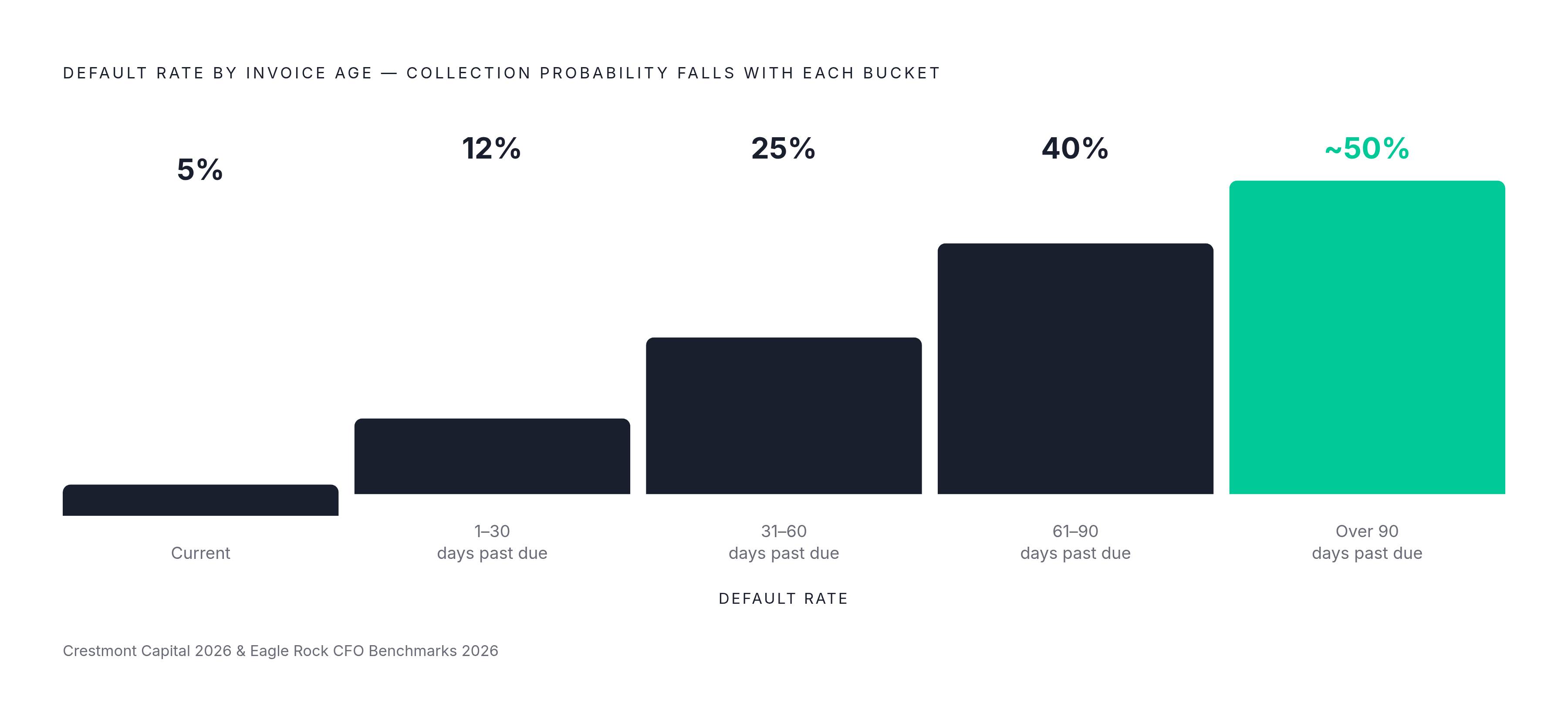
Once the schedule exists, the next step assigns a default percentage to each bucket, and those percentages climb as the buckets get older. Current invoices might carry a low estimated default rate. Invoices 90 days past due might carry something far higher. This escalation isn't a style choice. It mirrors the collection probability decay described earlier: the older the bucket, the worse the odds, the higher the rate assigned to it.

The math itself is simple multiplication followed by addition. Multiplying the total dollar amount in each bucket by that bucket's default percentage gives the estimated uncollectible amount for that bucket. Do that across every bucket, add the results together, and the sum is the required allowance balance, the total amount the company believes it will never collect.

One worked illustration spreads receivables across five buckets, with default rates climbing as high as 50% for the oldest category, and that produces a specific required allowance balance for the business in that example. The spread matters as much as the total. A company could have the exact same total receivables balance as a competitor and still need a much larger allowance, simply because more of its money is concentrated in the highest-default bucket than the lowest-default one.

The percentages themselves aren't pulled out of thin air. They come from the company's own historical collection data: what fraction of invoices in each bucket actually went uncollected in prior periods. That history makes the rates specific and defensible. A newer business without enough internal history to draw on can lean on industry-level benchmarks as a starting point, the way a new driver leans on a learner's permit before getting their own license. But the output of this step is a target. It's the balance the Allowance for Doubtful Accounts needs to reach, not yet the number that goes into the journal entry. That distinction trips up more people than almost anything else in this method, and it deserves its own section.

Recording bad debt expense: why the adjusting entry is not the full allowance amount

The required allowance balance calculated in the previous step, which causes the most confusion in the aging method, is not the bad debt expense recorded for the period. Bad debt expense equals the required ending allowance balance minus whatever balance the Allowance for Doubtful Accounts already carries.

Picture two scenarios. In the first, the Allowance for Doubtful Accounts starts the period with a debit balance, meaning prior write-offs exceeded prior estimates and the account is sitting in the hole. The adjusting entry in this case has to cover both the new required balance and that existing shortfall, so the expense recorded is larger than the aging schedule's raw estimate.

In the second scenario, the allowance already holds an existing credit balance going into the period, maybe from a prior period's estimate that hasn't been fully used up yet. Here, the adjusting entry only needs to record the gap between the new required balance and what's already sitting in the account. If the aging analysis calls for a certain allowance and the account already carries a smaller existing credit balance, the adjusting entry books only the difference in bad debt expense, not the full required allowance.

The takeaway: the aging method is always targeting a balance on the balance sheet, not calculating an expense directly from scratch each period. That's the mechanical feature that separates it from the percentage of sales method, which does compute the expense directly as a flat rate against revenue. Aging works backward from where the allowance needs to end up.

The write-off entry itself, which happens when a specific account gets confirmed as a lost cause, debits Allowance for Doubtful Accounts and credits Accounts Receivable. That entry does not touch total assets, and it does not touch the income statement. A contra-asset account and its paired receivable shrink by the same amount at the same time, so the net realizable value of receivables doesn't move an inch. The expense already got recorded back when the estimate was made. The write-off is just bookkeeping catching up to a loss that was already priced in.

Balance sheet and income statement effects

Everything calculated so far lands in two places on the financial statements, and they tell two different stories. Bad debt expense flows onto the income statement, where it reduces net income for the period. The Allowance for Doubtful Accounts flows onto the balance sheet, where it sits as a contra-asset and pulls gross accounts receivable down to its net realizable value, the amount the company actually expects to collect in cash.

A reader of the financials should care more about net realizable value than about the gross receivables number. Gross AR tells you how much customers owe on paper. Net realizable value tells you how much of that is actually coming. A business with a large gross receivables balance and a thin allowance looks healthier than one with a properly sized allowance reflecting a messier customer base, even if the second business has a far more accurate picture of its own cash position. The allowance is what keeps the balance sheet honest.

The aging method gets classified as a balance sheet approach for this reason. It optimizes for getting the allowance balance and the net realizable value right, rather than optimizing for matching expense to revenue in the period the way the percentage of sales method does. One sentence on the matching principle, since it matters but doesn't need a full tour here: percentage of sales ties bad debt expense directly to the revenue that generated it, which is a cleaner match for income statement purposes, while aging accepts a slightly less clean match in exchange for a more accurate balance sheet.

Consider a company running a slim net profit margin. Writing off a single meaningful bad debt at that kind of margin requires many multiples of brand-new revenue just to replace the lost profit. An understated allowance doesn't just create an accounting headache down the line. It misrepresents how much the company is actually earning, right now, to anyone reading the balance sheet, including lenders and investors who are making decisions based on it.

Comparison with percentage of sales and specific identification

Three methods exist for estimating bad debt, and each one is built to optimize for something different, not to outrank the others.

Percentage of sales applies a single rate to revenue for the period and prioritizes matching expense to revenue cleanly on the income statement. It's fast, it's simple, and it works well for businesses with a fairly stable, homogeneous customer base where bad debt tracks revenue predictably.

Percentage of receivables applies one flat rate to the entire gross accounts receivable balance, regardless of how old any individual invoice is. AccountingTools has called this flat version "not sufficiently refined," since it treats a recently issued invoice the same as one far past due, even though the latter is in obviously worse shape.

The aging method solves that exact problem by disaggregating receivables into buckets and assigning differentiated rates to each one. That makes it the most granular of the three approaches. It also makes it the most labor-intensive, requiring the business to build and maintain the aging schedule.

Some businesses don't pick just one. A common hybrid approach uses the aging method for the bulk of receivables, where bucketing is efficient, and switches to specific identification for a handful of large or unusually risky accounts that deserve individual scrutiny. That combination captures the speed of bucketing most of the portfolio while still giving the biggest, riskiest invoices the close look they warrant. None of these three methods is the "right" one in isolation. The right one depends on the size of the receivables portfolio, how diverse the customer base is, and how much time a finance team can reasonably spend on the estimate each period.

The CloudStream Case and the Stakes of Method Choice

The choice between these methods isn't a theoretical exercise for an accounting exam. A CPA Exam Mastery case study, involving a company called CloudStream, shows just how different the output can be.

CloudStream's accounting team had been using the percentage of sales method. When they switched to the aging method instead, the required allowance estimate jumped to approximately $23,000. The jump happened because a meaningful chunk of CloudStream's receivables had aged well beyond their due dates, and you couldn't see that age profile under the simpler, sales-based calculation. Percentage of sales looks at revenue and applies a blended historical rate. It has no mechanism for noticing that a specific pile of invoices has gone stale.

The gap between the two estimates wasn't a rounding error. It represented real cash exposure that CloudStream had been carrying on its books at an understated level, which meant management, lenders, and investors had all been looking at a rosier picture than the company's actual collections situation supported.

The practical lesson sits right on the surface of this case: when a company's receivables are aging and collections are genuinely slowing down, the aging method will catch it, because it's built to look at exactly that. A single blended rate applied to revenue has no eyes for it. That gap between what a method can see and what it can't is where the aging method earns its keep, and it's also where its own limitations start to matter.

The real limitations of the aging method: stale percentages, CECL compliance, and industry variation

The aging method is only as good as the percentages feeding it. Those default rates get built from historical collection data, and history has an expiration date. A recession, a shift in customer mix, or a new competitor stealing a company's best-paying clients can all change collection behavior faster than the historical rates reflect. A business running percentages calibrated to a calm economic stretch can end up badly underestimating losses the moment conditions turn, simply because the past stopped being a reliable guide to the present.

Bucket width adds another layer of judgment. If you build a 30-day bucket structure for a wholesale distributor with 60-day payment terms, it will miscategorize risk constantly, lumping together invoices that are actually fine with invoices that are already in trouble. Buckets need to be calibrated to how the specific business actually collects, not copied from a generic template.

Regulatory expectations have also shifted the ground under this whole method. Newer credit loss accounting standards push companies toward forward-looking loss estimates instead of estimates built purely on historical averages, so the aging method's traditional backward-looking percentages may need adjustment to stay compliant, depending on the entity and the accounting framework it falls under.

Industry variation also shapes how the aging method plays out. A 90-day-old invoice in construction, where payment cycles routinely stretch long, might carry a very different real-world default risk than a 90-day-old invoice in a business that normally collects in two weeks. The aging method gives every business the same structural approach, a schedule, a set of buckets, a default rate per bucket, but the actual numbers inside that structure have to be built from each company's own collection reality, not borrowed wholesale from somewhere else.