Cash Flow Forecasting with AR Data

Late Payments Are Normal; Your Forecast Probably Doesn't Know That Yet.

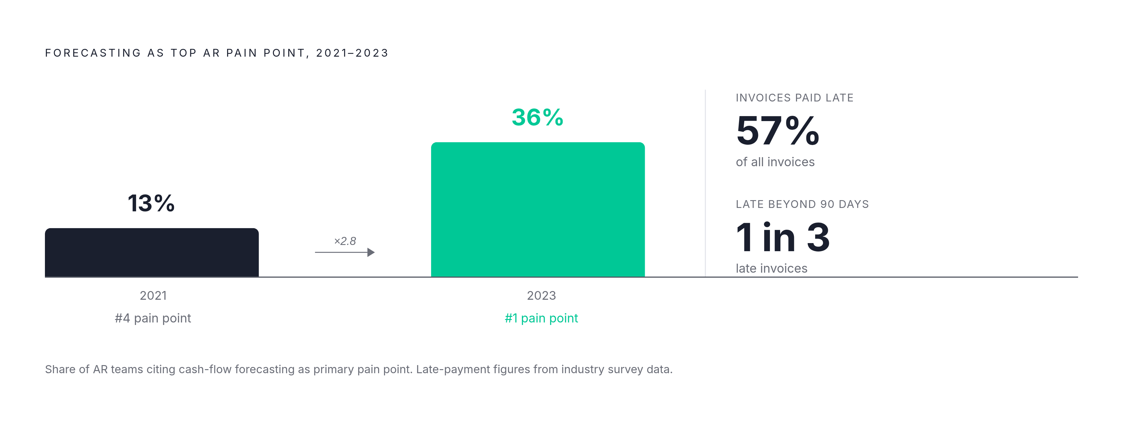
Late payments are not a surprise. They are the norm. Around 57% of invoices are paid late, and a third of those take more than 90 days to settle. If you are building a cash flow forecast on invoice due dates, you are not forecasting. You are hoping.

Here is the honest version of what most forecasts actually are: a spreadsheet that assumes customers pay when they say they will, stitched together by someone who knows better but lacks better data. Forecasting became the number one pain point in the AR process in 2023. That same metric was around 13% in 2021 and nearly tripled in two years. Meanwhile, well over half of organizations were still forecasting cash flows manually going into the mid-2020s, and a majority of U.S. businesses pointed to outdated methods as the top reason their forecasts were failing.

Finance leaders know forecasting matters more than ever. The inputs feeding those forecasts, though? Largely unchanged. The tool got more important. The raw material stayed exactly the same.

Fixing the forecast means fixing what feeds it. That means reading AR data differently.

The Scale of Late Payments and What It Costs a Forecast Built on Assumptions

Let me put some numbers to what "late payments are normal" actually means for a business trying to plan around its cash.

The average annual cost from late payments runs around $39,000 per company. One in ten companies absorbs over $100,000 in related expenses. And the majority of small business failures trace back to poor cash flow management. Late payments are not just a collections nuisance; they are an existential forecasting problem.

When the majority of invoices do not behave as modeled, any forecast built on due dates is systematically wrong before anyone even runs it. That is a structural miscalculation baked into the methodology. Not a one-off error. It is not bad luck. It is a known flaw that gets treated like an inconvenience.

Here is the real implication: a forecast is not just a planning tool. It is an early-warning system. And late-payment patterns are the signal it should be reading. A customer with net-30 terms who reliably pays on day 45 looks completely fine in an aging report right up until the cash fails to arrive when you needed it to. By then, you are not forecasting anything. You are scrambling to cover the gap you should have seen coming.

The structural reasons most forecasts miss this signal are not accidents. They are features of how the models are built.

Three Structural Reasons Most AR-Based Forecasts Produce Unreliable Numbers

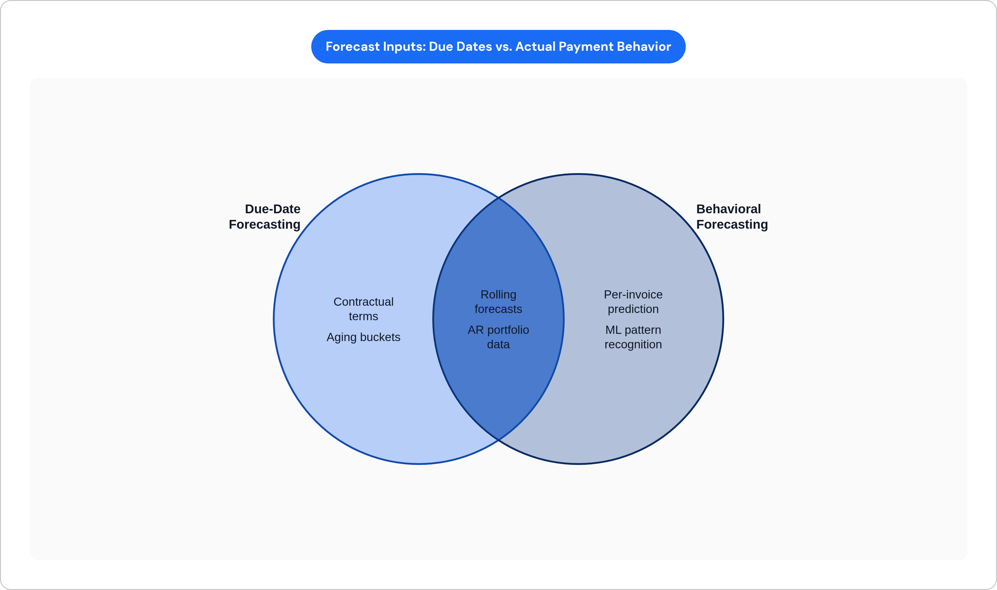
You can blame the model all you want. But the model is usually not the problem. The inputs are.

They are reading the wrong data point. An aging report shows what is owed. It does not tell you when the money will actually arrive. Due dates are contractual. Pay dates are behavioral. Only one of them tells you what your bank account will look like next Thursday, and it is not the one most forecasts are built on.

The AR data feeding the model is stale before it even gets there. Remittances sitting unprocessed in inboxes. Deductions logged in spreadsheets nobody updates in real time. Open invoice balances in the ERP that do not reflect what happened last Tuesday. A significant share of CFOs admit they do not fully trust the accuracy of their own financial data. That credibility problem starts upstream of any forecast model, and no amount of modeling sophistication fixes it downstream. You cannot model your way out of bad inputs.

They are ignoring forward-looking signals entirely. FX rates shift. Commodity prices move. Customer industries run into headwinds. These signals change payment behavior before the change shows up in the ledger. If the only data you are reading is historical AR, you are always a few weeks behind the actual story.

The operational cost of this is real. Treasury teams spend hundreds of hours annually generating cash flow forecasts. Not because forecasting is inherently that hard; because the inputs are broken and require constant human intervention to manage. That time is not rigor. It is compensation for bad data, and most teams have just accepted that as the job.

The Four Main Methods for Forecasting AR and Where Each One Breaks Down

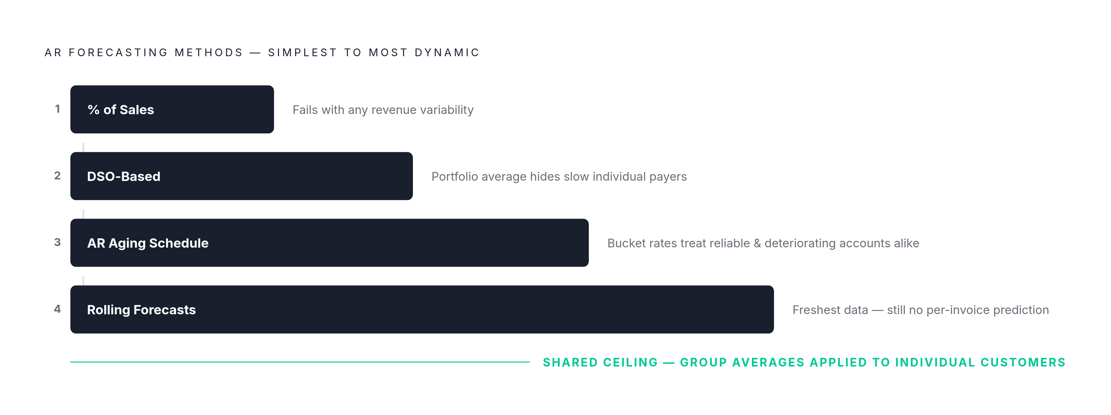
These are the four approaches most finance teams use. All of them have legitimate uses. All of them have a ceiling, and the ceiling is lower than most people think.

DSO-based forecasting takes your days sales outstanding and multiplies it against a revenue estimate. Useful as a portfolio-level benchmark. A DSO under 45 days generally signals healthy collection velocity. Above 60 typically means friction somewhere in the process. But DSO is a single average, and a portfolio sitting at a 48-day DSO still hides customers who pay at 75 days. The average looks fine. The cash does not arrive on time. You find out the hard way.

AR aging schedule method sorts outstanding invoices into 30-day buckets and applies historical collection rates per bucket. If 85% of your 0-to-30-day AR historically gets collected and that bucket holds $10 million, you forecast $8.5 million in expected inflow. Clean and intuitive. The limitation is that a collection rate is still an average. It does not distinguish between a reliable customer with a one-time delay and a customer whose payment behavior is genuinely deteriorating. Both land in the same bucket. Both get the same rate applied. One of them is lying to you.

Percentage-of-sales method assumes AR stays a stable percentage of revenue over time. It works for businesses with highly predictable, non-seasonal revenue. For anything variable, it falls apart almost immediately.

Rolling forecasts update continuously as new AR and sales data comes in, capturing seasonal shifts through quarter-over-quarter comparisons. This is the most practical traditional method for maintaining current accuracy. It is still operating on aggregated data, but at least the aggregated data is fresh.

The shared limitation across all four is this: they run on averaged or aggregated inputs. None of them generate a per-invoice prediction grounded in that specific customer's actual payment history. They are applying group assumptions to individual customers. And individual customers do not behave like groups. That gap between the assumption and the reality is where forecast error lives.

What Invoice-Level Prediction Changes About Forecasting Accuracy

Here is where things get genuinely different.

Invoice-level cash prediction generates a predicted payment date and payment probability for each individual open invoice. Instead of applying a collection rate to an aging bucket, you are asking a more specific question: when will this customer pay this invoice, based on how they have actually behaved in the past?

The logic is straightforward. Customer-specific behavioral predictions, aggregated across the full AR portfolio, produce a more accurate total than portfolio-wide averages applied uniformly. Academic research has validated this per-invoice approach, proposing statistical methods for predicting time-to-payment using behavioral data. But honestly, experienced AR practitioners already know this intuitively. You know which customers always pay late. You know which ones will call to dispute before the ink is dry. The question is whether your forecast knows it too, or whether it is still treating every open invoice as equally likely to arrive on time.

What this method surfaces that aggregate approaches consistently miss:

• A customer's actual payment velocity, not their contracted terms
• The behavioral difference between a first-time payer and a habitually slow one
• Early signals of change before they show up in aggregate metrics

Here is a concrete example. A customer who normally pays early has started paying at the last possible moment across three consecutive invoices. An aggregate DSO model sees no change; the average still looks fine. A per-invoice model flags the drift immediately. It is nothing, or it is a liquidity problem developing on their end. Either way, you want to know before they stop paying entirely, not after the missed payment shows up in your next monthly report.

The output from invoice-level prediction is a cash inflow curve with meaningful confidence intervals. Not a single due-date-based number. Not a bucket average. A probability-weighted view of when cash is actually expected to land. This is the point where AR data stops being a historical record and starts functioning as a forward signal.

How Machine Learning Improves on Manual Per-Invoice Prediction at Scale

Manual per-invoice prediction is possible for a small AR portfolio. At any real scale, it becomes untenable fast. This is where machine learning earns its place in the conversation.

ML models trained on two or more years of AR history generate per-invoice payment predictions more accurately than bucket-level averages, and they do it across thousands of invoices simultaneously. More importantly, they track things a static aging report cannot:

• Payment velocity changes over time
• Communication patterns, including dispute frequency and response lag
• Subtle shifts in account activity that precede payment delays
• Behavioral signals that do not appear in ERP data at all

Think of it this way. A good AR collector who has worked the same accounts for five years knows which customers are going to be a problem before the invoice is even due. They have pattern recognition built from experience, from a hundred small signals that never make it into a spreadsheet. ML is doing the same thing, just across a portfolio too large for any one person to hold in their head. It is not magic; it is pattern recognition at scale, applied consistently, without the collector needing to catch every account on a good day.

The working capital payoff is not abstract. Research consistently shows that meaningful gains in forecast accuracy free up working capital that was previously held as a precautionary buffer. A company with $100 million in revenue and a 55-day DSO unlocks real, material capital by shaving even 10 days off that number. That is not a rounding error. That is a capital allocation decision that changes what you can actually do with the business.

And yet the gap between what finance leaders say they need and what they have actually deployed remains wide. Nearly nine in ten finance leaders say predictive analytics is critical for their AR software. The expectation is there. The implementation still lags. That gap is costing them real money.

Why Forecast Accuracy Depends on Collections Data Being Live, Not Static

A forecast is only as current as the AR data feeding it. Static ERP exports become stale the moment collections activity moves. This sounds obvious. It is also widely ignored, partly because the workarounds have become so normalized that nobody notices them anymore. People have been patching the same leak for years and started calling it the plumbing.

The operational blockers that degrade data freshness in practice:

• Remittances sitting unprocessed in email inboxes for days
• Invoices stuck inside supplier portals like Coupa or Ariba, logged there but not reflected in the ERP
• Missing documents, a W-9, a purchase order number, a tax certificate, that freeze payment workflows entirely
• Disputes batched and entered manually at the end of the week instead of logged in real time

Companies that achieve strong quarterly forecasting accuracy share one thing in common: they integrate collections processes directly with their forecasting models. Collections timing is not a downstream output. It is an input.

This reframes the problem usefully. Forecasting accuracy is a collections execution problem as much as it is a modeling problem. If follow-up is slow or inconsistent, the AR data flowing into the forecast is incomplete. Incomplete data produces confident-looking numbers that are wrong. And wrong numbers that look confident are worse than uncertain numbers that are honest, because at least uncertain numbers make you go check.

Companies relying on manual processes take significantly longer to follow up on overdue accounts than those using AR automation. That delay creates forecast blind spots. Not because the model is broken; because the signal never arrived in the first place.

What "live" data actually means in practice is not glamorous:

• Cash application processed in real time, not batched
• Open invoice status updated as customer interactions happen
• Disputes logged immediately, not at end of week
• Portal-logged payment confirmations reflected in the ERP without a manual sync

None of that is technically exotic. Most of it is just process discipline. But process discipline at scale requires tooling that makes the disciplined path the easiest path. Otherwise, people batch things at the end of the week because that is what fits into their day, and the forecast quietly falls behind.

Practical Steps Finance Teams Can Take to Improve Forecast Accuracy with Existing AR Data

You do not need a complete system overhaul to start moving the needle. Most finance teams already have the raw material. AR data is sitting there. The problem is usually that nobody is reading it correctly, or nobody built the habit of reading it in a way that actually feeds the forecast.

Stop using due dates as the primary forecast input. Replace them with historical pay date data per customer or customer segment. The due date is a contractual fiction. The actual pay date is the data that matters.

Segment AR before applying collection rate assumptions. Customer size, industry, payment history, and terms all produce meaningfully different behavioral profiles. A blanket collection rate applied across all customers obscures real variance. Segment first, then apply rates appropriate to each group.

Move from static aging snapshots to rolling forecasts. Update as new payment data comes in. Monthly batch updates miss behavioral drift that develops week by week. A customer who has slipped from paying at day 32 to day 41 to day 50 over three payment cycles will look fine in a monthly report; a rolling model catches it.

Identify and close the data gaps creating stale AR. Work backward from the forecast to find where the data breaks down. Unprocessed remittances. Portal invoices not reflected in the ERP. Deductions in spreadsheets nobody touches until month-end. These are specific, fixable problems. Fix the specific ones first, because trying to fix them all at once is how nothing gets fixed.

Build a 13-week cash flow forecast as the core short-term liquidity tool, but stress-test its AR inputs. The 13-week model is the standard for short-term cash visibility. Its reliability depends entirely on the AR data quality feeding it. A well-structured 13-week model on bad AR data is a precise-looking wrong answer.

Introduce forward-looking inputs alongside historical AR data. FX rates, customer credit signals, commodity price exposure. These catch payment behavior shifts before they appear in aging reports. Aging data is a lagging indicator; forward signals are leading indicators. Both belong in the model, and right now most teams are only using one of them.

The math on why this is worth the effort is simple. A 1-point accuracy gain in forecasting unlocks meaningfully more deployable cash at any revenue scale. Most small businesses have less than four months of operating cash on hand. That is not a lot of room to be wrong. And a lot of teams are being wrong in ways that are entirely preventable, with data they already have, using habits they could build starting next week.